Eigenfaces for Dummies

 

Author: Jer Ming Chen

Date: 06/07/2011, UCLA Class Project

 

Abstract:

This project is aim to implement facial recognition using Singular Value Decomposition (SVD) that has being widely used as the basis of facial recognition algorithms. The eigen-vectors of SVD over the facial dataset are often regarded as eigenfaces. Due to human resources, time constraint, and level of experiences, this project does not try to innovate from the baseline method. The core of this project is to learn the algorithm and implemented it.

The environment which my project runs on is .Net Framework 4.0. This is a Microsoft platform independent environment. Meaning my project can be run on any computer with .Net installed, which includes non-Windows machines. Please look for third party implementations of the platform if you are not using Windows. The project is programmed in C# and WPF with additional 3rd party classes: IL Numerics.net [1] for SVD calculations and ShaniSoft [2] for reading PGM image files reliably. Both classes are free. IL Numerics.net uses CPU optimizations for calculations, thus, doing analysis on IL Numerics.net is a good choice for .NET developers.

Most researchers use MATLAB, Octave, or “R” for numeric analysis. There are also newer offering such as F# and “Sho” for numeric analysis. This paper uses C# environment instead. As you can see, I need extra binary library to handle numeric analysis because C# is not built for this specific task.

Compare to other websites that explained eigenfaces, I will try to explain how to perform facial recognition and reconstructions as simple as possible. You will see more pseudo code instead of math notations. In addition, you will see some little details that are often left out from other sources.

 

Introduction:

I am going to bluntly list out the sites I find useful if you wish to read more about it.

- http://en.wikipedia.org/wiki/Eigenface [3]

- http://www.scholarpedia.org/article/Eigenfaces [4]

- http://www.pages.drexel.edu/~sis26/Eigenface%20Tutorial.htm [5]

- http://openbio.sourceforge.net/resources/eigenfaces/eigenfaces-html/facesOptions.html [6]

Facial recognition is often done in Google Picasa, Microsoft Live Gallery, and Facebook. To allow computer recognize a person is not only useful for casual users, but, very convenient to identify person of interest for police or military uses. One way to achieve this is by feature extractions. Eigenfaces can be understood as feature faces. Eigenfaces is a basic facial recognition introduced by M. Turk and A. Pentland [9] in 1991. It is not the most accurate method compares to the modern approaches, but, it sets the basis for many new algorithms in the field.

What does it mean by feature faces? What feature are we tracking? In this paper, we don’t know exactly what features we are tracking, we only know that we are tracking important features. We obtain the important features by using Singular Value Decomposition (SVD) over covariance matrix.

 

Singular Value Decomposition (SVD):

SVD is one of common way to perform Principal Component Analysis (PCA). PCA in short is a process to find important contributors of data. Thus, instead of considering all possible contributors to a result, we only use the important ones. This not only reduced a lot of calculation on the remaining important contributors, but, it also saved a lot of memory used to perform analysis. SVD over covariance matrix has the following characteristics:

• You will get U S V* from the decomposition.
• The U and V contain eigen-vectors ordered from highest variance to lowest variance.
• Highest variance means the vector captures features that change the most.
• Eigen-vectors are orthogonal to each other. They don’t share the same features.
• Eigen-values in S indicate the importance of each corresponding eigen-vector.

In summary, SVD will tell you which special vector that give you’re the most “diverse” result from your dataset, and less important vectors in descending orders. Meaning the first column of the eigen-vectors are the most important, the second column of eigen-vectors are the second most important, and so on.

Here is an image from Wikipedia, which explains how SVD is performed.

In here we want to keep U as eigen-vectors. Eigenfaces are simply colored eigen-vectors converted to an image; yellow being the largest vector and red being the second largest vector. We will have tons of vectors/eigenfaces; we only need the top K of them as they describe most of the facial features.

 

Steps to Create Eigenfaces:

 

1) Load your training faces.

You can get faces from PubFig: Public Figures Face Database [7] and LFWcrop Face Dataset [8]. The second site offers a cropped version from the first site. You can also get your faces from other place.

This part is completely up to you. I am using gray scaled faces from LFWcrop Face Dataset [8] website. They are in PGM file format, which I used ShaniSoft ‘s class object to read the file for me. It is not very difficult to read the file myself, but, I prefer to use existing solutions to avoid introducing new bugs. Existing solutions usually provides a more reliable and more efficient solution than we can do it ourselves.

I also include a feature to convert color BMP, JPEG, and GIF into gray scale images, although it is slower than reading already gray scaled images.

 

2) Convert your images into column vectors.

Put your image pixels in an array and put it in a column of matrix. If you have 30 faces, you will have 30 columns. If your face has 100 gray scaled pixels, you will have 100 rows.

Now your matrix should have [Image1, Image2, Image3 …., ImageM].

Image1 Pixel 1	Image2 Pixel 1	Image3 Pixel 1	Image4 Pixel 1	.....	ImageM Pixel 1
Image1 Pixel 2					ImageM Pixel 2
Image1 Pixel 3					ImageM Pixel 3
.....					.....
.....					.....
Image1 Pixel N	Image2 Pixel N	Image3 Pixel N	Image4 Pixel N	.....	ImageM Pixel N

 

3) Calculate the mean.

Image you merged all your columns into one column. Thus, you will add all “Images Columns” pixel-by-pixel or row-by-row. And then, it is divided by M total images. You should have a single column which contains the mean pixels. This is what we called “Mean Face”.

Now your column should have:

Mean Image Pixel 1

Mean Image Pixel 2

Mean Image Pixel 3

.....

.....

Mean Image Pixel N

 

4) Reduce your matrix created in step2 using mean from step3.

For each column in matrix, subtract each image pixel value by mean pixel.

WHY? Before we can perform SVD, we need to have the data centered at origin. After that, we can perform matrix rotation and scaling shown from the above image. Matrix rotation and scaling are performed at center of the coordinate system, thus, we need to move our dataset to the center.

 

5) Calculate Covariance Matrix C

C = (A)(A_Transpose) where A is your matrix from step4.

I did this in IL Numerics Library. Remember if you are using IL Numeric, converting 2x2 array from C# will get a transpose of your original array. Make sure you double check that you have correct pixelCount-by-imageCount matrix dimension.

Covariance Matrix vs. Correlation Matrix In statistics field, using correlation matrix is preferred as there is no bias to the columns. In here, we don't need to use correlation matrix because our covariance matrix is the same as correlation matrix. This is because all our columns are in the same range of 0 to 255 gray scale values. If our columns have different range, then, we need to normalize it, which is one step in correlation matrix.

 

6) Calculate SVD on matrix C.

There is not much to say, we use the algorithm provided from the existing library, such as svd(Matrix C). You can implement SVD yourself, but, it is not recommended. Using existing library would have a much faster, more accurate, more reliable, and less resources consuming solution than we implementing it from scratch.

In here, we use U as eigen-vector.

 

7) Alternative Methods.

Doing 5 and 6 when you have more pixels and fewer images, it will be slower. This is because we will have N² = pixelCount * pixelCount matrix to calculate, which is much slower compare to a much smaller M² = imageCount * imageCount matrix to calculate. Often you will have more pixels than images, thus, you can use this alternative method presented by M. Turk and A. Pentland [9]. If you have more images, then, you use step 5 and 6.

The argument is that we only need to keep M number of eigen-vectors to capture most of the features. Thus, even though we didn't use the entire N number of eigen-vectors, it is enough. In addition, often we use less eigen-vectors than M as well.

7.1)

Instead of creating covariance matrix

C = (A)(A_Transpose)

We do

C_small = (A_Transpose)(A)

7.2)

Perform SVD on C_small.

In here, use V as eigen-vector "temporarily". We need to do extra work to get the desired eigen-vectors because we didn’t use the step5 and step6.

7.3)

Create a new eigneValuesPowerNHalf by

eigneValuesPowerNHalf = eigenValues^(-0.5)

7.4)

Create new eigen-vector that we actual want.

For each eigenvectorV[i]

matrixMultiplied[i] = (A)(eigenvectorV[i])

eigenVectorU[i] = matrixMultiplied[i] / eigneValuesPowerNHalf [i]

End loop

eigenVectors U are the eigen-vectors we want.

7.5)

Normalize eigen-vectors using vector mean. This is often implicitly described in other papers.

For each eigenVectorU[i] in eigenVectorU

For each valueA in eigenVectorU[i]

sumOfSquares = sumOfSquares + valueA^2

End loop

vectorMean = SquareRoot(sumOfSquares)

eigenVectorU[i] = eigenVectorU[i] / vectorMean

End loop

Now we should have M amount of normalized eigen-vectors U.

 

8) Visualize Eigenfaces.

Now you should have normalized eigen-vectors from step6 or step7. To create the image, you need to scale it properly. The smallest value in your vector should be converted to 0. Largest value should be converted to 255. Any value in between should be scaled within the min-max range.

For example, newPixel[i] = 255 * (eigenVectorPixel[i] – min) / (max – min)

 

9) Reconstructing Faces.

First we compute weight W[i] of the new input face for each EigenVector[i].

We do this by doing dot product of new face column and eigen-vector column. It is the same as doing matrix multiplication with transpose of eigen-vector. We will get a single scalar W[i] per eigen-vector[i].

Because eigen-vectors are normalized, we simply multiply the W[i] to EigenVector[i] and added to mean face. Note that we are adding mean face because we subtracted mean face at step4. In order to get the actual face, we need to add mean face back.

In here, we can see that we can reconstruct any untrained faces using existing eigen-vectors as long as we have enough training faces and enough eigen-vectors. The orientations of the faces are not affected here.

 

10) Recognition.

We use the same technique from step9 to calculate the W weights. We obtain weights for input image and the trained images from our dataset. There are many always to calculate the distance. One simple way is using Euclidean distance where we

1. Calculate sum of square of scaled down difference.
   • sum(square( ( difference of each W[i] ) / pixel count ))
   • Notice we scaled down the weight difference by pixel count, so larger pictures would still have the same scale.
2. We take a square root of the sum.
3. Divide it by square root of (amount of vectors used).
   • Similar to previous argument. When we use more eigen-vectors, the distance is scaled up by it. Thus, we need to scale it back down. Since we are using Euclidean distance, the scale is square root of dimensions.

We use Euclidean distance because each vector is orthogonal to each other. If the vectors are not orthogonal to each other, we cannot use this approach.

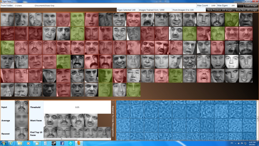
My program returns the top10 result of the images that consider being close enough to the existing trained images. The threshold is default to 0.05, but, you can change it any time you like in the provided GUI. However, I do not recommend increasing the threshold as it will return faces that are not similar enough to the input face. In the "Want Faces" row, the row contains all the images trained for the selected person. Because this program will train more than one faces per person if applicable, the program will have better accuracy on recognition.

However, note that the faces used in this project are not suitable for recognition because faces have different orientations and facial expressions. The algorithm is one of the early facial recognition techniques. It only has adequate recognition result using more constrained images, such as passport photos where the faces are facing the same direction and only have single type of facial expressions. There are other techniques to solve these types of problems, such as Fisherface[10] or Kernel Eigenfaces [11], but, that’s outside of this project’s objective.

 

Result:

My program will train the first image of a person. A person is identified by the file name. A file name with more than two character differences are consider different name. Other images are trained with probability of 20%.

	Faces in gray are first image of a person, thus, will always be trained.
	Faces in green are randomly sampled training faces.
	Faces in red are not trained.

My project supports PGM, BMP, JPEG, and GIF. There may be other image format supported, but, that's up to .NET 2.0 System.Drawing.Bitmap's capability. I recommend to use PGM because other formats are slower. If you have gray images in formats other than PGM, it will first randomly samples 10 pixels and determine if the image is in gray scale. If it is gray scaled, the program will use red channel as the gray scale values. If it is color image, it will spend more time on converting each pixel to gray scale; it is using 0.3, 0.59, 0.11 scaling factors instead of naive average. This is because human vision is more sensitive to one color over another. For more information about gray scale conversion, please refer to Wikipedia grayscale [12].

My program will train, reconstruct, and find the selected image/person. If you select gray or green faces, the program is expected to retrieve the exact same face from the training set. If you select red faces, try to select more eigenfaces if the result is not desirable.

 

Dataset 2:

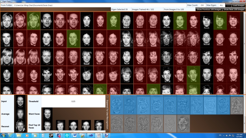
As described earlier, the baseline method is more suitable for more constrained images. Psychological Image Collection at Stirling[13] offers a good selection of faces. This database is capable of providing desired faces based on my queries. Thus, this source is much more flexible in obtaining the faces needed. One drawback of this source is the image dimensions are off by few pixels, thus, I need to correct them beforehand. The file names are also modified for my program as well. If you wish to get the same faces, you can download it from above "Dataset 2".

As shown above, each person has three expressions. Each person has at least one image trained and other faces are randomly trained.

In here, I demonstrated the algorithm is much better at recognition when everyone is facing in the same directions. The expression is not a big problem in this case. This is mainly because their expressions are not dramatically different from other expressions. An expression with mouth wide open would be much dramatic than the expressions shown.

 

Conclusion:

This project demonstrated eigenfaces in simple steps. It used different software solution to compute numeric analysis instead of using typical software package such as MATLAB or Octave. The program is able to reconstruct untrained images. This allows the application to generate new faces without too much data being stored. The program is then attempted to match top10 images that are consider similar to the input image. In here, I demonstrated the weakness of this algorithm as it is not suitable when faces are in different orientations. I also demonstrated the program using another dataset where everyone faces the same direction, which yields much better recognition accuracy than the previous dataset.

 

References:

[1] Numeric Analysis Library for .NET IL Numerics.net

[2] Reading PGM file for .NET ShaniSoft

[3] Eigenface from Wikipedia http://en.wikipedia.org/wiki/Eigenface

[4] Eigenface from Scholarpedia http://www.scholarpedia.org/article/Eigenfaces

[5] Eigenface Tutorial http://www.pages.drexel.edu/~sis26/Eigenface%20Tutorial.htm

[6] Eigenface Tutorial http://openbio.sourceforge.net/resources/eigenfaces/eigenfaces-html/facesOptions.html

[7] Face dataset PubFig: Public Figures Face Database

[8] Crop version of face dataset LFWcrop Face Dataset

[9] Eigenfaces for Recognition (using smaller faster matrix) M. Turk and A. Pentland (1991)

[10] Better recognition, Fisherface (Belhumeur et al. 1997)

[11] Better recognition, Kernel Eigenfaces (Yang 2002)

[12] Grayscale from Wikipedia http://en.wikipedia.org/wiki/Grayscale

[13] Psychological Image Collection at Stirling http://pics.psych.stir.ac.uk/

 

 

© 2024 - jmcspot.com